Project 3 diabetes_data: High_School_Graduate Analysis
Jasmine Gallaway and Keren Vivas 2023-11-16
1. Introduction section
The data analyzed in this report is derived from the Diabetes Health Indicators Dataset, which was gathered through the Behavioral Risk Factor Surveillance System (BRFSS) in the year 2015. The BRFSS is an annual health-related telephone survey conducted by the Centers for Disease Control and Prevention (CDC). This dataset encompasses a substantial collection of over 200,000 survey responses, featuring 21 distinct variables or factors, along with a pivotal response variable termed “Diabetes_binary.” This response variable comprises three discrete levels:
0 = No diabetes or diabetes only during pregnancy. 1 = Prediabetes. 2 = Established diabetes.
The dataset encompasses a diverse array of variables that cover a wide spectrum of information, including the current diabetes status of the survey respondents, various demographic details, physical and mental health metrics, dietary habits, and lifestyle factors. The specific variables selected for analysis in this report are as follows:
- Demographics: This category includes two categorical variables: “Age” and “Sex” of the respondents.
- Physical Conditions: These variables encompass “HighBP,” “HighChol,” and “HeartDiseaseorAttack.” These are categorical variables, taking values of 0 or 1, indicating the presence or absence of high blood pressure, high cholesterol, and a history of heart disease or heart attacks. Additionally, the “Body Mass Index (BMI)” is included as a continuous variable, with values ranging from 12 to 98, providing insights into the respondents’ body composition.
- Mental Conditions: The variable “MentHlth” is a continuous variable that quantifies the number of days in a month during which the respondent’s mental health was not good. It ranges from 1 to 30.
- Diet Conditions: Two categorical variables, “Fruits” and “Veggies,” denote whether respondents consume fruits and vegetables one or more times per day. These variables take values of 1 (indicating consumption) or 0 (indicating non-consumption).
- Habits: This category includes two categorical variables: “Smoker” and “PhysActivity.” “Smoker” indicates whether respondents have smoked at least 100 cigarettes in their lifetime (with values 1 for yes and 0 for no), while “PhysActivity” assesses whether respondents have engaged in physical activity within the last month (with values 1 for yes and 0 for no).
The Exploratory Data Analysis (EDA) of the selected variables is designed to offer a holistic understanding of the health and lifestyle characteristics of the survey respondents. This preliminary phase of analysis helps us uncover patterns within the data.
Subsequently, when we move to modeling the data, our objective is to delve deeper and gain insights into the intricate ways these factors impact an individual’s diabetes status. Our analysis will not only reveal the influence of these factors but also quantify the individual contributions of each factor to the risk of diabetes.
In the end, the entire analysis will be segmented based on the level of education. This segmentation enables us to investigate how this specific demographic factor influences the overall findings. By doing so, we can discern whether educational levels play a significant role in shaping the relationship between health, lifestyle, and diabetes risk.
2. Required packages section
#Reading in libraries
library(readr)        #For reading
library(dplyr)        #For data manipulation
library(ggplot2)      #For plotting
library(caret)        #For modeling
library(rmarkdown)    #For creating of dynamic documents
library(purrr)        #For data manipulation
library(glmnet)       #For Lasso model
library(randomForest) #For random forest model
library(gbm)          #Fors boosting model
library(Metrics)      #For logLoss()
library(cvms)         #For cross-validation
library(rpart)        #For tree model
library(pls)          #For Partial Least Squares Model
3. Data section
In this section we change most of the variables into factors and label them with appropriate names.
#readin data
diabetes_data <- read_csv("diabetes_binary_health_indicators_BRFSS2015.csv")

#making a tibble
diabetes_data <- as_tibble(diabetes_data)

#changing diabetes_binary to factor
diabetes_data$Diabetes_binary <- diabetes_data$Diabetes_binary %>%
  factor(levels = c(0,1),
         labels = c("No","Pre"))

#combine education levels one and two
diabetes_data$Education <- diabetes_data$Education %>%
  factor(levels = c(1,2,3,4,5,6),
            labels = c("Elementary", "Elementary", "Some_High_School", "High_School_Graduate", "Some_College", "College_Graduate"))

#changing sex to factor
diabetes_data$Sex <- diabetes_data$Sex %>%
  factor(levels = c(0,1),
         labels = c("female", "male"))

#changing age to factor
diabetes_data$Age <- diabetes_data$Age %>%
  factor(levels = c(1,2,3,4,5,6,7,8,9,10,11,12,13),
         labels = c("18-24", "25-30", "31-35", "36-40", "41-45", "46-50", "51-55", "56-60", "61-65", "66-70", "71-75", "76-80", "80+"))

#Changing fruit to factor
diabetes_data$Fruits <- diabetes_data$Fruits %>%
  factor(levels = c(0, 1),
         labels = c("None", "Yes"))

#Changing physical activity to factor
diabetes_data$PhysActivity <- diabetes_data$PhysActivity %>%
  factor(levels = c(0, 1),
         labels = c("None", "Yes"))

#Changing smoker to factor
diabetes_data$Smoker <- diabetes_data$Smoker %>%
  factor(levels = c(0, 1),
         labels = c("No", "Yes"))

#Changing stroke to factor
diabetes_data$Stroke <- diabetes_data$Stroke %>%
  factor(levels = c(0, 1),
         labels = c("No", "Yes"))

#Changing heart disease or attack to factor
diabetes_data$HeartDiseaseorAttack <- diabetes_data$HeartDiseaseorAttack %>%
  factor(levels = c(0, 1),
         labels = c("No", "Yes"))

#Changing veggies to factor
diabetes_data$Veggies <- diabetes_data$Veggies %>%
  factor(levels = c(0, 1),
         labels = c("None", "Yes"))

#Changing Heavy alcohol consumption to factor
diabetes_data$HvyAlcoholConsump <- diabetes_data$HvyAlcoholConsump %>%
  factor(levels = c(0, 1),
         labels = c("No", "Yes"))

#Changing any healthcare to factor
diabetes_data$AnyHealthcare <- diabetes_data$AnyHealthcare %>%
  factor(levels = c(0, 1),
         labels = c("No", "Yes"))

#Changing nodocbcCost to factor
diabetes_data$NoDocbcCost <- diabetes_data$NoDocbcCost %>%
  factor(levels = c(0, 1),
         labels = c("No", "Yes"))

#Changing GenHlth to factor
diabetes_data$GenHlth <- diabetes_data$GenHlth %>%
  factor(levels = c(1, 2, 3, 4, 5),
         labels = c("Excellent", "Very Good", "Good", "Fair", "Poor"))

#Changing DiffWalk to factor
diabetes_data$DiffWalk <- diabetes_data$DiffWalk %>%
  factor(levels = c(0, 1),
         labels = c("No", "Yes"))

#changing HighBP to factor
diabetes_data$HighBP <- diabetes_data$HighBP %>%
  factor(levels = c(0, 1),
         labels = c("No", "Yes"))

#changing HighChol to factor
diabetes_data$HighChol <- diabetes_data$HighChol %>%
  factor(levels = c(0,1),
         labels = c("No", "Yes"))

#changing CholCheck to factor
diabetes_data$CholCheck <- diabetes_data$CholCheck %>%
  factor(levels = c(0,1),
         labels = c("No", "Yes"))

#changing Income to factor
diabetes_data$Income <- diabetes_data$Income %>%
  factor(levels = c(1,2,3,4,5,6,7,8),
         labels = c("Less than $10k", "$10k to less than $15k", "$15kto less than $20k", "$20k to less than $25k", "$25k to less than $35k", "$35k to less than $50k", "$50k to less than $75k", "$75k or more"))
Below our data set is subset into the specified education level for the page.
# Subset data into a single Education level
subset_data <- diabetes_data %>%
 filter(Education == params$Education)
4. Summarizations section
Below is some initial exploratory data analysis on the dataset. We began
with looking at group summaries of BMI and mental health. Both are
grouped by the Diabetes_binary variable which sorts the participants
into no diabetes, prediabetes, or diabetes.
#gathering summary statistics of BMI
sum_data1 <- subset_data %>%
  group_by(Diabetes_binary) %>%
  summarize(mean = mean(BMI),
            sd = sd(BMI),
            min = min(BMI),
            max = max(BMI),
            IQR = IQR(BMI))
#printing out
print(sum_data1)
## # A tibble: 2 × 6
##   Diabetes_binary  mean    sd   min   max   IQR
##   <fct>           <dbl> <dbl> <dbl> <dbl> <dbl>
## 1 No               28.4  6.43    12    98     7
## 2 Pre              32.1  7.42    13    92     9
#Summary statistics of mental health
sum_data2 <- subset_data %>%
  group_by(Diabetes_binary) %>%
  summarize(mean = mean(MentHlth),
            sd = sd(MentHlth),
            min = min(MentHlth),
            max = max(MentHlth))
print(sum_data2)
## # A tibble: 2 × 5
##   Diabetes_binary  mean    sd   min   max
##   <fct>           <dbl> <dbl> <dbl> <dbl>
## 1 No               3.45  7.83     0    30
## 2 Pre              4.72  9.15     0    30
Contingency Tables
After initial group summaries we then made several contingency tables in order to observe some of the possible relationships between variables. Based on these contingency tables we were able to numerically see where some trends might occur.
 #1-way contingency table
 one_way_table <- table(subset_data$Fruits)
 one_way_table
##
##  None   Yes
## 27011 35739
 #2-way contingency table
 two_way_table <- table(subset_data$Smoker, subset_data$HighChol)
 two_way_table
##
##          No   Yes
##   No  16828 12599
##   Yes 16961 16362
 #3-way contingency table
 three_way_table <- table(subset_data$HighBP, subset_data$HighChol, subset_data$HeartDiseaseorAttack)
 three_way_table
## , ,  = No
##
##
##          No   Yes
##   No  20678  8648
##   Yes 10876 15081
##
## , ,  = Yes
##
##
##          No   Yes
##   No    834   870
##   Yes  1401  4362
#4 Contingency table for diabetes_binary vs no doctors visits because of cost
 tbl_four <- table(subset_data$NoDocbcCost, subset_data$Diabetes_binary)
 tbl_four
##
##          No   Pre
##   No  46595  9837
##   Yes  5089  1229
#5 Contingency table for diabetes_binary vs general health ratings
 tbl_five <- table(subset_data$GenHlth, subset_data$Diabetes_binary)
 tbl_five
##
##                No   Pre
##   Excellent  6959   265
##   Very Good 16840  1630
##   Good      17715  4133
##   Fair       7514  3477
##   Poor       2656  1561
#6 Contingency table for diabetes_binary vs NoDocbcCost vs GenHlth
 tbl_six <- table(subset_data$GenHlth, subset_data$Diabetes_binary, subset_data$NoDocbcCost)
 tbl_six
## , ,  = No
##
##
##                No   Pre
##   Excellent  6593   244
##   Very Good 15768  1544
##   Good      15891  3770
##   Fair       6284  3023
##   Poor       2059  1256
##
## , ,  = Yes
##
##
##                No   Pre
##   Excellent   366    21
##   Very Good  1072    86
##   Good       1824   363
##   Fair       1230   454
##   Poor        597   305
Plots
We then looked at some additional combinations of variables in graphs to observe other relationships within the data. In these plots we are attempting to graph possible relationships between variables. If any trends are found it could give insight to which variables are important to use in our predictive modeling.
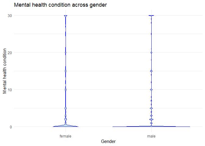
#Plot 1 is a violin plot that illustrates the distribution of the Mental Health variable across the two sex categories, female and male.

plot1 <- ggplot(subset_data, aes(x = Sex, y = MentHlth)) +
  geom_violin(fill = "lightblue", color = "blue", alpha = 0.7) +
  labs(title = "Mental health condition across gender", x = "Gender", y = "Mental health condition") +
  theme_minimal()
print(plot1)
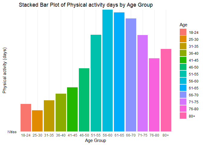
#Plot 2 is a stacked bar plot that depicts the distribution of the Physical Activity variable across all age groups, with each group represented by a different color.

plot2 <- ggplot(data = subset_data, aes(x = Age, y = PhysActivity , fill = Age)) +
  geom_bar(stat = "identity") +
  labs(title = "Stacked Bar Plot of Physical activity days by Age Group", x = "Age Group", y = "Physical activity (days)") +
  theme_minimal()
print(plot2)
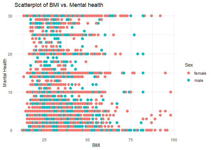
#Plot 3 is a scatter plot designed to visualize the relationship between the Body Mass Index (BMI) and Mental Health variables, with points colored by sex (female and male)

plot3 <- ggplot(subset_data, aes(x = BMI, y = MentHlth)) +
  geom_point(aes(color = Sex), size = 3) +
  labs(title = "Scatterplot of BMI vs. Mental health", x = "BMI", y = "Mental Health") +
  theme_minimal()
print(plot3)
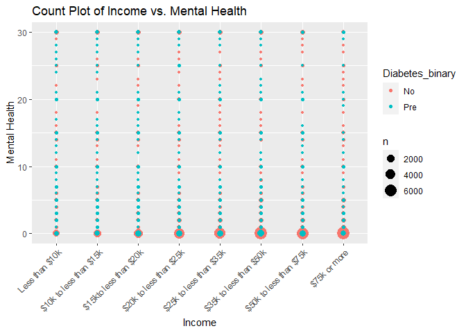
#Plot 4 is a count plot of income versus mental health and color coded by the response variable of Diabetes_binary
plot4 <- ggplot(subset_data, aes(x = Income, y = MentHlth)) +
  geom_count(aes(color = Diabetes_binary)) +
  labs(title = "Count Plot of Income vs. Mental Health", x = "Income", y = "Mental Health") +
  theme(axis.text.x = element_text(angle = 45, vjust = 1, hjust=1))
print(plot4)
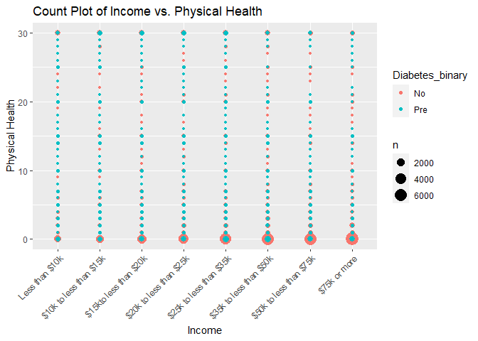
#Plot 5 is a count plot of income versus physical health and color coded by the response variable of Diabetes_binary
plot5 <- ggplot(subset_data, aes(x = Income, y = PhysHlth)) +
  geom_count(aes(color = Diabetes_binary)) +
  labs(title = "Count Plot of Income vs. Physical Health", x = "Income", y = "Physical Health") +
  theme(axis.text.x = element_text(angle = 45, vjust = 1, hjust=1))
print(plot5)
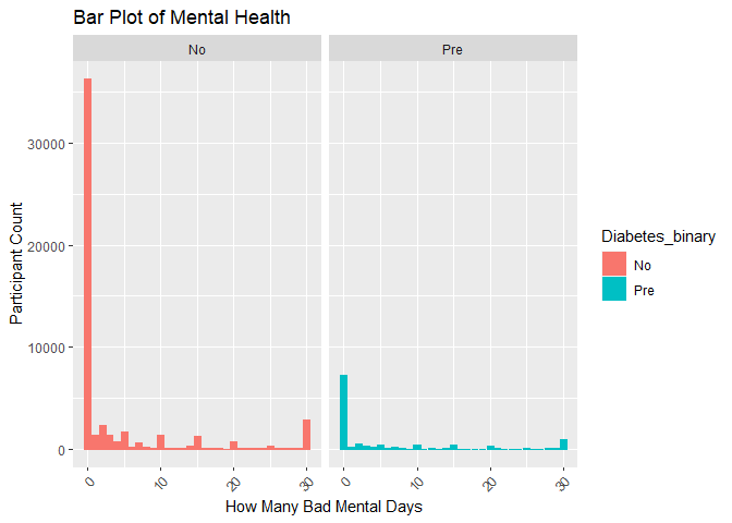
#Plot 6 is a bar plot of diabetes_binary versus mental health used to uncrowd the graphs
plot6 <- ggplot(subset_data, aes(x = MentHlth)) +
  geom_bar(aes(color = Diabetes_binary, fill = Diabetes_binary)) +
  facet_wrap(~Diabetes_binary) +
  labs(title = "Bar Plot of Mental Health", x = "How Many Bad Mental Days", y = "Participant Count") +
  theme(axis.text.x = element_text(angle = 45, vjust = 1, hjust=1))
print(plot6)
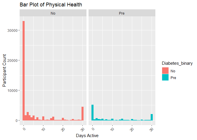
#Plot 7 is a bar plot of diabetes_binary versus physical health used to uncrowd the graphs
plot7 <- ggplot(subset_data, aes(x = PhysHlth)) +
  geom_bar(aes(color = Diabetes_binary, fill = Diabetes_binary)) +
  facet_wrap(~Diabetes_binary) +
  labs(title = "Bar Plot of Physical Health", x = "Days Active", y = "Participant Count") +
  theme(axis.text.x = element_text(angle = 45, vjust = 1, hjust=1))
print(plot7)
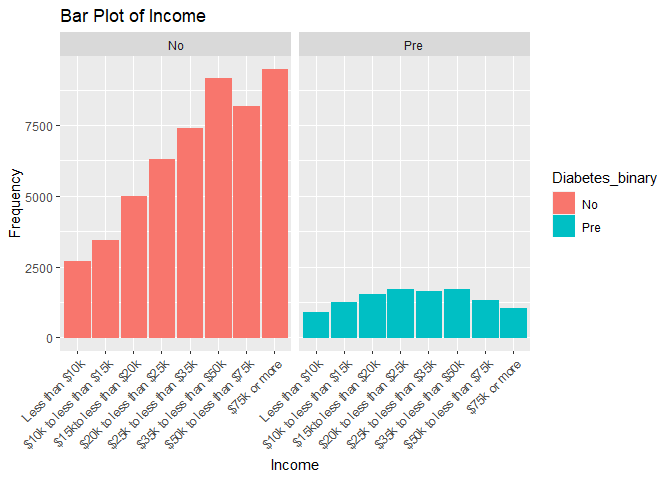
#Plot 8 is a bar plot of diabetes_binary versus income used to uncrowd the graphs
plot8 <- ggplot(subset_data, aes(x = Income)) +
  geom_bar(aes(color = Diabetes_binary, fill = Diabetes_binary)) +
  facet_wrap(~Diabetes_binary) +
  labs(title = "Bar Plot of Income", x = "Income", y = "Frequency") +
  theme(axis.text.x = element_text(angle = 45, vjust = 1, hjust=1))
print(plot8)
5. Modeling
Below begins the work to shift into modeling our data. We had some
initial issues with modeling due to our labeling of the variables. We
also had some modeling issues due to there being no recorded responses
of 2 / “Diabetes” within the Diabetes_binary dataset. Due to this lack
of response, the “Diabetes” level of Diabetes_binary had to be removed
in order for the models to work. The code chunk directly below removes
that factor level. Some of the variables we arbitrarily chose to focus
on in our modeling are Sex, Income, Age, BMI, MentHlth, PhysHlth,
HighBP, Fruits, HvyAlcoholConsump, and NodocbcCost. Variable selection
can be done with penalization modeling such as LASSO.
#Dropping level
subset_data$Diabetes_binary <- droplevels(subset_data$Diabetes_binary)

#Setting seed for reproducibility
set.seed(3033)

#Splitting the data
intrain <- createDataPartition(y = subset_data$Diabetes_binary, p= 0.7, list = FALSE)

#Splitting the data
training <- subset_data[intrain,]
testing <- subset_data[-intrain,]

#Smaller training set for computations
training <- training[1:250,]
What log loss is and why we may prefer it to things like accuracy?
Logarithmic loss is metric used to evaluate how well a model fits. Also
known as cross-entropy loss, log loss is used on binary classification
models where the responses are either 0 or 1. Log loss calculates the
difference between the predicted probabilities and the actual values.
The lower the log loss value, the better the fit of the model is to the
data. Log loss is preferred with this data set because of our focus on
the binary response of diabetes. Our Diabetes_binary response variable
has three responses of no diabetes, prediabetes, and diabetes; however,
there seems to be no recorded response of the factor level of 2
(diabetes) within the data so the recorded responses are either 0 or 1.
Log loss is better than accuracy in this case because log loss focuses
on models that predict the class better and penalizes models that are
further from the class.
What a LASSO logistic regression model is and why we might try to use this over basic logistic regresion?
LASSO (Least Absolute Shrinkage and Selection Operator) is a type of regularized logistic regression. It adds a penalty term to the logistic regression’s likelihood function to encourage feature selection by driving some coefficients to exactly zero. This can improve model interpretability and reduce overfitting and that is why it is used over the basic logistic regresion.
LASSO logistic regression is a valuable tool when you have high-dimensional datasets with potentially redundant or irrelevant features. It can improve model performance, reduce overfitting, and enhance model interpretability by automatically selecting the most relevant predictors while eliminating the least important ones. However, the choice between basic logistic regression and LASSO logistic regression depends on the specific characteristics of your data and the goals of your analysis.
Fit a LASSO logistic regression model and choose the best model
#Setting control for the train control
control <- trainControl(method = "cv", number = 5, classProbs = TRUE, summaryFunction = mnLogLoss)

#Fitting a LASSO logistic regression model
model_lasso <- train(Diabetes_binary ~ Sex + Income + Age + BMI + MentHlth + PhysHlth + HighBP + Fruits + HvyAlcoholConsump + NoDocbcCost,
  data = training,
  method = "glmnet",
  trControl =control,
  tuneGrid = expand.grid(alpha = 1, lambda = seq(0.001, 1, length = 100))
)

#Predict
pred_model_lasso <- predict(model_lasso, newdata = testing, type = "prob")

#Turn values into 1's and 0's for the log loss calculation
testing$Diabetes_binary <- ifelse(testing$Diabetes_binary == "No", 0, 1)

# LogLoss function with explicit conversion to numeric
LogLoss <- function(actual, predicted) {
  result <- -1 / length(actual) * sum((actual * log(predicted) + (1 - actual) * log(1 - predicted)))
  return(result)
}

# Calculate log loss on the testing set
test_logloss_lasso <- LogLoss(testing$Diabetes_binary, pred_model_lasso)

test_logloss_lasso
## [1] 2.16225
# Display the log loss on the testing set
cat("Log Loss on Testing Set:", test_logloss_lasso, "\n")
## Log Loss on Testing Set: 2.16225
what a classification tree model is and why we might try to use it?
A classification tree, specifically known as a decision tree for classification, is a model designed for classifying data. It recursively divides the input space into regions, assigning a class label to each region. The decision-making process is visualized as a tree structure, where internal nodes represent decisions based on specific features, branches depict the outcomes of those decisions, and leaf nodes contain the final predicted classes. The construction of a classification tree involves selecting optimal features to split the data at each internal node, with the process continuing until a stopping criterion is met, such as a maximum tree depth or a minimum number of samples in a leaf node. The tree’s depth and complexity are controlled by different values of the complexity parameter, typically determined through cross-validation to select the best parameter.
We might choose to use a classification tree for several reasons. It offers benefits such as excellent interpretability, no assumption of linearity, handling of both numeric and non-numeric data, automatic variable selection, insensitivity to feature scale, robustness to outliers, suitability for imbalanced data, and its role as a building block for ensemble methods, enhancing predictive performance.
Fit a classification tree with varying values for the complexity parameter and choose the best model (best complexity parameter)
#Set seed for reproducibility
set.seed(123)

# Create 5-fold cross-validation indices
folds <- createFolds(training$Diabetes_binary, k = 5, list = TRUE, returnTrain = FALSE)

# Create a grid of complexity parameter values to try
cp_values <- seq(0.01, 0.1, by = 0.01)

# Create a data frame to store log loss for each complexity parameter
logloss_df <- data.frame(cp = numeric(length(cp_values)), logloss = numeric(length(cp_values)))

# Loop through different complexity parameters
for (i in seq_along(cp_values)) {
  avg_logloss <- 0

  # Perform 5-fold cross-validation
  for (fold in seq_along(folds)) {
    # Extract training and validation sets
    training_set <- training[-folds[[fold]], ]
    validation_set <- training[folds[[fold]], ]

    # Build the classification tree on the training set
    tree_model <- rpart(Diabetes_binary ~ Sex + Income + Age + BMI + MentHlth + PhysHlth + HighBP + Fruits + HvyAlcoholConsump + NoDocbcCost, data = training_set, method = "class", control = rpart.control(cp = cp_values[i]))

    # Make predictions on the validation set
    predictions <- predict(tree_model, newdata = validation_set, type = "prob")[, 2]

    # Calculate log loss on the validation set
    fold_logloss <- logLoss(as.numeric(validation_set$Diabetes_binary) - 1, predictions)

    avg_logloss <- avg_logloss + fold_logloss
  }

  # Calculate average log loss over all folds
  avg_logloss <- avg_logloss / length(folds)

  # Store average log loss in the data frame
  logloss_df[i, ] <- c(cp = cp_values[i], logloss = avg_logloss)
}

# Find the best complexity parameter with the minimum average log loss
best_cp <- logloss_df$cp[which.min(logloss_df$logloss)]

# Build the final classification tree with the best complexity parameter
final_tree_model <- rpart(Diabetes_binary ~ Sex + Income + Age + BMI + MentHlth + PhysHlth + HighBP + Fruits + HvyAlcoholConsump + NoDocbcCost, data = training, method = "class", control = rpart.control(cp = best_cp))

# Display the best complexity parameter
cat("Best Complexity Parameter:", best_cp, "\n")
## Best Complexity Parameter: 0.08
# Display the final tree
print(final_tree_model)
## n= 250
##
## node), split, n, loss, yval, (yprob)
##       * denotes terminal node
##
## 1) root 250 58 No (0.7680000 0.2320000) *
# Evaluate the final model on the testing set
test_predictions <- predict(final_tree_model, newdata = testing, type = "prob")[, 2]

# Calculate log loss on the testing set
test_logloss_tree <- abs(logLoss(as.numeric(testing$Diabetes_binary) - 1, test_predictions))

# Display the log loss on the testing set
cat("Log Loss on Testing Set:", test_logloss_tree, "\n")
## Log Loss on Testing Set: 0.7220256
What a bagged CART model is?
A bagged CART (Bootstrap Aggregating for Classification and Regression Trees) model is an ensemble machine learning technique aimed at enhancing predictive model stability and accuracy while mitigating overfitting. The process involves creating multiple bootstrap samples from the original dataset by randomly selecting data points with replacement. Each bootstrap sample is used to train an independent CART model (decision tree). The predictions from all individual trees are then combined to form the final ensemble prediction. For classification tasks, the mode of predictions is often used, while the average is employed for regression problems. Bagging creates diversity in the models by training them on different subsets of the data, making the ensemble more robust and less prone to overfitting.
Fit a bagged CART and choose the best model
#Changing factor levels for eased calculations
testing$Diabetes_binary <- factor(testing$Diabetes_binary, levels = c(0, 1), labels = c("No", "Pre"))

#Setting control for the train control
control <- trainControl(method = "cv", number = 5, classProbs = TRUE, summaryFunction = mnLogLoss)

# Fit a bagged model (using bagged trees) on the training data
model_bagged <- train(Diabetes_binary ~ Sex + Income + Age + BMI + MentHlth + PhysHlth + HighBP + Fruits + HvyAlcoholConsump + NoDocbcCost, data = training, method = "treebag", trControl = control)

# Predict probabilities on the testing set
pred_probabilities <- predict(model_bagged, newdata = testing, type = "prob")

# Turn values into 1's and 0's for the log loss calculation
testing$Diabetes_binary <- as.numeric(testing$Diabetes_binary) - 1

pred_prob_pre <- pred_probabilities[,"Pre"]

# LogLoss function with epsilon to avoid log(0)
LogLoss <- function(actual, predicted) {
  epsilon <- 1e-15  # Small epsilon value to avoid log(0)

  # Add epsilon to avoid log(0) or log(1)
  predicted <- pmax(pmin(predicted, 1 - epsilon), epsilon)

  result <- -1 / length(actual) * sum((actual * log(predicted) + (1 - actual) * log(1 - predicted)))
  return(result)
}
# Calculate log loss on the testing set
test_logloss_cart <- LogLoss(testing$Diabetes_binary, pred_prob_pre)

test_logloss_cart
## [1] 0.7746904
# Display the log loss on the testing set
cat("Log Loss on Testing Set:", test_logloss_cart, "\n")
## Log Loss on Testing Set: 0.7746904
What a logistic regression is and why we apply it to this kind of data?
Logistic regression is a form of predictive analysis in which the
regression models the relationship(s) of a binary response variable to
one or more other variables. Typically we think of linear regression
models, but generalized linear models, such as logistic regression, are
used in cases in which the general assumptions of linear models are
broken. The general assumptions of a linear model are that the model is
for a continuous response, errors are normally distributed, and that
constant variance can be assumed. In this case our Diabetes_binary
variable could do well being modeled by logistic regression. In our data
Diabetes_binary has two recorded responses of either 0 “No diabetes”
or 1 “Prediabetes”; this is not a continuous response and therefore a
general linear model cannot be used. A typical logistic function can be
backsolved to result in showing what is called a link function. The link
function shows how a linear model could be fit to our response variable.
The link function of logistic regression is called the logit function
and models the log odds of success. The log odds of success is the
probability that the success (or 1 response) will occur. In this
scenario it feels wrong to call prediabetes a success; however, we will
statistically still consider 1 “Prediabetes” to be the success.
Fit 3 candidate logistic regression models and choose the best
#Setting trainControl to include cv
my_ctrl <- trainControl(method = "cv", number = 5, classProbs = TRUE, summaryFunction = mnLogLoss)

# Model 1: Logistic Regression with first set of predictors
model1 <- train(Diabetes_binary ~ Age + BMI + HighBP, data = training,
                method = "glm",
                trControl = my_ctrl,
                metric = "logLoss",
                family = binomial(link = "logit"))

#Saving logLoss value
m1 <- model1$results$logLoss

#Observing Summaries
model1
## Generalized Linear Model
##
## 250 samples
##   3 predictor
##   2 classes: 'No', 'Pre'
##
## No pre-processing
## Resampling: Cross-Validated (5 fold)
## Summary of sample sizes: 200, 200, 200, 199, 201
## Resampling results:
##
##   logLoss
##   0.4922877
# Model 2: Logistic Regression with different predictor variables
model2 <- train(Diabetes_binary ~ Age*PhysActivity, data = training,
                method = "glm",
                trControl = my_ctrl,
                metric = "logLoss",
                family = binomial(link = "logit"))

#Saving logLoss value
m2 <- model2$results$logLoss

#Observing Summaries
model2
## Generalized Linear Model
##
## 250 samples
##   2 predictor
##   2 classes: 'No', 'Pre'
##
## No pre-processing
## Resampling: Cross-Validated (5 fold)
## Summary of sample sizes: 199, 200, 201, 199, 201
## Resampling results:
##
##   logLoss
##   0.6617013
# Model 3: Logistic Regression with more parameter variations
model3 <- train(Diabetes_binary ~ Age + PhysActivity + HvyAlcoholConsump + Fruits, data = training,
                method = "glm",
                trControl = my_ctrl,
                metric = "logLoss",
                family = binomial(link = "logit"))

#Saving logLoss value
m3 <- model3$results$logLoss

#Observing Summaries
model3
## Generalized Linear Model
##
## 250 samples
##   4 predictor
##   2 classes: 'No', 'Pre'
##
## No pre-processing
## Resampling: Cross-Validated (5 fold)
## Summary of sample sizes: 201, 201, 200, 199, 199
## Resampling results:
##
##   logLoss
##   0.5808374
#Making a table to compare the logLoss metric values and pick the smallest value
comparing <- c(Model1 = m1, Model2 = m2,Model3 = m3)
best_logistic_model <- names(which.min(comparing))
best_logistic_model
## [1] "Model1"
#building a contender item to automate returning the name of the model that worked the best
log_contender <- if (best_logistic_model == "Model1"){
           log_contender <- model1
           } else if (best_logistic_model == "Model2"){
           long_contender <- model2
           } else if (best_logistic_model == "Model3"){
           log_contender <- model3
}

#Prediction for contending logistic model with testing data
#Due to my model objects being train objects the actual predict function that R uses to run is predict.train which requires type = "prob" for classification problems
log_result <- predict(log_contender, newdata = testing, type = "prob")

#Saving the testing values as numerict so that they can be used for calculations
testing$Diabetes_binary <- as.numeric(testing$Diabetes_binary)

#Picking the pre (prediabetes) column to use in my logloss function
success_col <- log_result[,"Pre"]

#Creating a log loss function to compare the final results
LogLoss_values <- function(binary_num, pred)
{
 abs(-mean(binary_num * log(pred) + (1 - binary_num) * log(1 - pred)))
}

#Gathering the logLoss value of the predicted logistic candidate to compare to other models
logistic_logLoss <- LogLoss_values(testing$Diabetes_binary, success_col)
print(logistic_logLoss)
## [1] 0.7210212
# Display the log loss on the testing set
cat("Log Loss on Testing Set:", logistic_logLoss, "\n")
## Log Loss on Testing Set: 0.7210212
what a random forest is and why we might use it instead of a basic classification tree?
A random forest is another ensemble method of modeling. Random forests are similar to bagging in that both take bootstrapping samples from the data to build multiple trees. After repeat sampling and tree building, these ensemble tree building models can take the average or majority classification as their prediction. With our data being a classification problem, our random forest would take the class predicted by moajority of the trees it builds. Building many trees and then taking the average or majority vote decreases the variance that a basic classification tree would have which makes the ensemble methods the preferred model when prediction is the focus. Random forests differ from bagging as they take in a subset of the variables rather than using all of them for prediction. This subset increases bias, but also can decrease variance.
Fit a random forest model and choose the best model
Here it looks like we fit one overall model but our mtry value, which is the number of variables to sample from at each split in the tree, was a range of 1 to 3. This range is how we fitted multiple models into one overall train function. So here, in order to pick the best model, we have to look for the mtry value with the lowest logLoss value.
#setting control for the train control
control <- trainControl(method = "cv", number = 5, classProbs = TRUE, summaryFunction = mnLogLoss)

#Fitting a random forest model
rf_fit <- train(Diabetes_binary ~ Age + HvyAlcoholConsump + HighBP, data = training,
                method = "rf",
                trControl = control,
                metric = "logLoss",
                tuneGrid = expand.grid(mtry = 1:3))

#Saving the logloss value of mtry 1 as object
var1 <- rf_fit$results$logLoss[[1]]

#Saving the logloss value of mtry 2 as object
var2 <- rf_fit$results$logLoss[[2]]

#Saving the logloss value of mtry 3 as object
var3 <- rf_fit$results$logLoss[[3]]

#Making a table to compare the logLoss metric values and pick the smallest value
battle_of_logloss <- c(Mtry1 = var1, Mtry2 = var2, Mtry3 = var3)
best_rf_model <- names(which.min(battle_of_logloss))

best_rf_model
## [1] "Mtry3"
#building a contender item to automate returning the mtry tree that worked the best in the random forest model
rf_contender <- if (best_rf_model == "Mtry1"){
           rf_contender <- 1
           } else if (best_rf_model == "Mtry2"){
           rf_contender <- 2
           } else if (best_rf_model == "Mtry3"){
           rf_contender <- 3
           }

#Now to specify what training model (which mtry) should be used on the testing dataset
#We took the same format as above, but we automated the mtry value by inputting our winning rf_contender value
rf_best <- train(Diabetes_binary ~ Age + HvyAlcoholConsump + HighBP, data = training,
                method = "rf",
                trControl = control,
                metric = "logLoss",
                tuneGrid = expand.grid(mtry = rf_contender))

#Now we can train the testing dataset and predict with our rf_best model
rf_result <- predict(rf_best, newdata = testing)

#Turning values into 0 and 1 for the log loss calculation
testing$Diabetes_binary <- ifelse(testing$Diabetes_binary == "No", 0, 1)

#Picking the pre (prediabetes) column to use in my logloss function
pre_col <- ifelse(rf_result == "No", 0, 1)

#Reiterating the log loss function to compare the final results
#The 1e-15 is added in here because the results of the rf predictions are 0 and 1 and in the equation binary_num*log(pred) would result in Nan
LogLoss_values <- function(binary_num, pred)
{ abs(-mean(binary_num * log(pred + 1e-15) + (1 - binary_num) * log(1 - pred + 1e-15)))
}

#Gathering the logLoss value of the predicted logistic candidate to compare to other models
rf_logLoss <- LogLoss_values(testing$Diabetes_binary, pre_col)

print(rf_logLoss)
## [1] 32.00121
# Display the log loss on the testing set
cat("Log Loss on Testing Set:", rf_logLoss, "\n")
## Log Loss on Testing Set: 32.00121
What the Partial Least Squares model is?
Partial least squares(PLS) model is a dimension reduction techinque. PLS is similar to principal component analysis except that the reduction strategy used by PLS is driven by the response variable. PLS picks linear combinations of correlated variables that cover the most variability in the dataset to model as predictors. PLS is more difficult to interpret than logistic regression or a tree regression.
Fit models and choose the best model
#creating the control for the train model
control <- trainControl(method = "cv", number = 5, classProbs = TRUE, summaryFunction = mnLogLoss)

#Fitting a partial least squares model
pls_fit <- train(Diabetes_binary ~ Sex + BMI + HighChol + MentHlth + Fruits + NoDocbcCost, data = training,
                method = "kernelpls",
                trControl = control,
                metric = "logLoss")

#Saving the logloss value of mtry 1 as object
comp1 <- pls_fit$results$logLoss[[1]]

#Saving the logloss value of mtry 2 as object
comp2 <- pls_fit$results$logLoss[[2]]

#Saving the logloss value of mtry 3 as object
comp3 <- pls_fit$results$logLoss[[3]]

#Making a table to compare the logLoss metric values and pick the smallest value
battles_of_logloss <- c(Ncomp1 = comp1, Ncomp2 = comp2, Ncomp3 = comp3)
best_pls_model <- names(which.min(battles_of_logloss))

best_pls_model
## [1] "Ncomp3"
#building a contender item to automate returning the mtry tree that worked the best in the random forest model
pls_contender <- if (best_pls_model == "Ncomp1"){
           pls_contender <- 1
           } else if (best_pls_model == "Ncomp2"){
           pls_contender <- 2
           } else if (best_pls_model == "Ncomp3"){
           pls_contender <- 3
           }

#Now to specify what training model (which mtry) should be used on the testing dataset
#We took the same format as above, but we automated the mtry value by inputting our winning rf_contender value
pls_best <- train(Diabetes_binary ~ Sex + BMI + HighChol + MentHlth + Fruits + NoDocbcCost, data = training,
                method = "kernelpls",
                trControl = control,
                metric = "logLoss",
                ncmop = pls_contender)

#Now we can train the testing dataset and predict with our pls_best model
pls_result <- predict(pls_best, newdata = testing)

#Turning values into 0 and 1 for the log loss calculation
testing$Diabetes_binary <- ifelse(testing$Diabetes_binary == "No", 0, 1)


#Picking the pre (prediabetes) column to use in my logloss function
pre_col <- ifelse(pls_result == "No", 0, 1)

#Reiterating the log loss function to compare the final results
#The 1e-15 is added in here because the results of the rf predictions are 0 and 1 and in the equation binary_num*log(pred) would result in Nan
LogLoss_values <- function(binary_num, pred)
{ abs(-mean(binary_num * log(pred + 1e-15) + (1 - binary_num) * log(1 - pred + 1e-15)))
}

#Gathering the logLoss value of the predicted logistic candidate to compare to other models
pls_logLoss <- LogLoss_values(testing$Diabetes_binary, pre_col)

print(pls_logLoss)
## [1] 33.79934
# Display the log loss on the testing set
cat("Log Loss on Testing Set:", pls_logLoss, "\n")
## Log Loss on Testing Set: 33.79934
6. Final Model Selection (Compare the six best above and declare an overall winner)
What should happen is the tree or ensemble methods should be in the winning circle of the lowest log loss value. Ensemble methods run through multiple tree builds which should lower the variance of the model. With a lower variance there would hopefully be more predictice power. However, there are many tuning parameters that can be optimized and this report may not have the best fits overall.
#Lasso best model
Lasso <- test_logloss_lasso

#Bringing the tree best model
Tree <- test_logloss_tree

#Bringing the cart best model
Cart <- test_logloss_cart

#Bringing in the logistic best model
Logistic <- logistic_logLoss

#Bringing in the random forest model
Random <- rf_logLoss

#Bringing in the partial least squares model
Partial <- pls_logLoss

#Comparing the models
best_of_best <- c(Lasso_Model = Lasso, Tree_Model = Tree, Cart_Model = Cart, Logistic_Model = Logistic, Random_Forest_Model = Random, Partial_Least_Squares = Partial)
best <- names(which.min(best_of_best))

# Get the name or identifier of the best model
best_model <- paste(best)

# Print the result
cat("The best model is:", best_model, "with log loss:", best_of_best[best], "\n")
## The best model is: Logistic_Model with log loss: 0.7210212